How to Read Glm Output in R
Interpreting generalized linear models (GLM) obtained through glm is like to interpreting conventional linear models. Hither, nosotros will talk over the differences that need to be considered.
Basics of GLMs
GLMs enable the employ of linear models in cases where the response variable has an mistake distribution that is non-normal. Each distribution is associated with a specific approved link function. A link function \(g(ten)\) fulfills \(X \beta = g(\mu)\). For example, for a Poisson distribution, the canonical link function is \(1000(\mu) = \text{ln}(\mu)\). Estimates on the original scale can be obtained by taking the inverse of the link part, in this case, the exponential role: \(\mu = \exp(X \beta)\).
Data grooming
Nosotros will take 70% of the airquality samples for training and 30% for testing:
data(airquality) ozone <- subset(na.omit(airquality), select = c("Ozone", "Solar.R", "Current of air", "Temp")) set.seed(123) Due north.train <- ceiling(0.7 * nrow(ozone)) N.test <- nrow(ozone) - N.train trainset <- sample(seq_len(nrow(ozone)), N.train) testset <- setdiff(seq_len(nrow(ozone)), trainset) Grooming a GLM
For investigating the characteristics of GLMs, we will train a model, which assumes that errors are Poisson distributed.
By specifying family = "poisson", glm automatically selects the appropriate canonical link function, which is the logarithm. More information on possible families and their approved link functions tin be obtained via ?family.
model.pois <- glm(Ozone ~ Solar.R + Temp + Air current, data = ozone, family = "poisson", subset = trainset) summary(model.pois) ## ## Call: ## glm(formula = Ozone ~ Solar.R + Temp + Wind, family = "poisson", ## information = ozone, subset = trainset) ## ## Deviance Residuals: ## Min 1Q Median 3Q Max ## -4.0451 -2.4138 -0.8169 1.4265 eight.7946 ## ## Coefficients: ## Estimate Std. Error z value Pr(>|z|) ## (Intercept) 0.690227 0.218192 iii.163 0.00156 ** ## Solar.R 0.001815 0.000239 7.593 3.13e-14 *** ## Temp 0.043500 0.002295 18.956 < 2e-16 *** ## Wind -0.084244 0.005960 -xiv.134 < 2e-16 *** ## --- ## Signif. codes: 0 '***' 0.001 '**' 0.01 '*' 0.05 '.' 0.ane ' ' i ## ## (Dispersion parameter for poisson family taken to be ane) ## ## Null deviance: 1979.57 on 77 degrees of freedom ## Residual deviance: 530.51 on 74 degrees of freedom ## AIC: 951.97 ## ## Number of Fisher Scoring iterations: four In terms of the GLM summary output, there are the following differences to the output obtained from the lm summary function:
- Deviance (deviance of residuals / nil deviance / residue deviance)
- Other outputs: dispersion parameter, AIC, Fisher Scoring iterations
Moreover, the prediction office of GLMs is also a bit different. We volition beginning with investigating the deviance.
Deviance residuals
Nosotros already know residuals from the lm function. But what are deviance residuals? In ordinary least-squares, the rest associated with the \(i\)-th observation is defined equally
\[r_i = y_i - \hat{f}(x_i)\]
where \(\hat{f}(x) = \beta_0 + x^T \beta\) is the prediction part of the fitted model.
For GLMs, there are several means for specifying residuals. To understand deviance residuals, it is worthwhile to look at the other types of residuals first. For this, we define a few variables get-go:
expected <- ozone$Ozone[trainset] g <- family(model.pois)$linkfun # log function yard.inv <- family(model.pois)$linkinv # exp function estimates.log <- model.pois$linear.predictors # estimates on log scale estimates <- fitted(model.pois) # estimates on response scale (exponentiated) all.equal(thou.inv(estimates.log), estimates) ## [1] TRUE We volition cover 4 types of residuals: response residuals, working residuals, Pearson residuals, and, deviance residuals. At that place is likewise another type of residue chosen fractional residual, which is formed by determining residuals from models where individual features are excluded. This residual is not discussed here.
Response residuals
For blazon = "response", the conventional residue on the response level is computed, that is, \[r_i = y_i - \lid{f}(x_i)\,.\] This ways that the fitted residuals are transformed past taking the inverse of the link role:
# blazon = "response" res.response1 <- residuals(model.pois, type = "response") res.response2 <- expected - estimates all.equal(res.response1, res.response2) ## [1] TRUE Working residuals
For type = "working", the residuals are normalized past the estimates \(\hat{f}(x_i)\):
\[r_i = \frac{y_i - \chapeau{f}(x_i)}{\hat{f}(x_i)}\,.\]
# type = "working" res.working1 <- residuals(model.pois, type="working") res.working2 <- (expected - estimates) / estimates all.equal(res.working1, res.working2) ## [1] TRUE Pearson residuals
For blazon = "pearson", the Pearson residuals are computed. They are obtained past normalizing the residuals past the foursquare root of the approximate:
\[r_i = \frac{y_i - \hat{f}(x_i)}{\sqrt{\hat{f}(x_i)}}\,.\]
# type = "pearson" res.pearson1 <- residuals(model.pois, type="pearson") res.pearson2 <- (expected - estimates) / sqrt(estimates) all.equal(res.pearson1, res.pearson2) ## [i] TRUE Deviance residuals
Deviance residuals are divers by the deviance. The deviance of a model is given by
\[{D(y,{\hat {\mu }})=2{\Big (}\log {\big (}p(y\mid {\chapeau {\theta }}_{s}){\big )}-\log {\big (}p(y\mid {\hat {\theta }}_{0}){\big )}{\Big )}.\,}\]
where
- \(y\) is the result
- \(\hat{\mu}\) is the gauge of the model
- \(\hat{\theta}_s\) and \(\chapeau{\theta}_0\) are the parameters of the fitted saturated and proposed models, respectively. A saturated model has as many parameters as information technology has grooming points, that is, \(p = n\). Thus, it has a perfect fit. The proposed model can exist the any other model.
- \(p(y | \theta)\) is the likelihood of data given the model
The deviance indicates the extent to which the likelihood of the saturated model exceeds the likelihood of the proposed model. If the proposed model has a good fit, the deviance volition exist small. If the proposed model has a bad fit, the deviance will be high. For case, for the Poisson model, the deviance is
\[D = ii \cdot \sum_{i = i}^n y_i \cdot \log \left(\frac{y_i}{\lid{\mu}_i}\right) − (y_i − \hat{\mu}_i)\,.\]
In R, the deviance residuals correspond the contributions of individual samples to the deviance \(D\). More specifically, they are defined as the signed square roots of the unit deviances. Thus, the deviance residuals are coordinating to the conventional residuals: when they are squared, we obtain the sum of squares that we use for assessing the fit of the model. Nevertheless, while the sum of squares is the residual sum of squares for linear models, for GLMs, this is the deviance.
How does such a deviance expect like in practice? For example, for the Poisson distribution, the deviance residuals are defined equally:
\[r_i = \text{sgn}(y - \hat{\mu}_i) \cdot \sqrt{2 \cdot y_i \cdot \log \left(\frac{y_i}{\hat{\mu}_i}\correct) − (y_i − \hat{\mu}_i)}\,.\]
Let u.s.a. verify this in R:
# type = "deviance" res.dev1 <- residuals(model.pois, type = "deviance") res.dev2 <- residuals(model.pois) poisson.dev <- function (y, mu) # unit of measurement deviance 2 * (y * log(ifelse(y == 0, 1, y/mu)) - (y - mu)) res.dev3 <- sqrt(poisson.dev(expected, estimates)) * ifelse(expected > estimates, 1, -i) all.equal(res.dev1, res.dev2, res.dev3) ## [1] TRUE Note that, for ordinary least-squares models, the deviance residual is identical to the conventional rest.
Deviance residuals in practice
We can obtain the deviance residuals of our model using the residuals role:
summary(residuals(model.pois)) ## Min. 1st Qu. Median Mean 3rd Qu. Max. ## -4.0451 -ii.4138 -0.8169 -0.1840 1.4265 8.7946 Since the median deviance balance is close to zero, this means that our model is not biased in 1 direction (i.eastward. the out come is neither over- nor underestimated).
Null and rest deviance
Since nosotros have already introduced the deviance, understanding the nada and residual deviance is non a challenge anymore. Let us repeat the definition of the deviance in one case once more:
\[{D(y,{\hat {\mu }})=2{\Big (}\log {\big (}p(y\mid {\hat {\theta }}_{southward}){\large )}-\log {\big (}p(y\mid {\hat {\theta }}_{0}){\large )}{\Big )}.\,}\]
The null and residual deviance differ in \(\theta_0\):
- Null deviance: \(\theta_0\) refers to the naught model (i.east. an intercept-only model)
- Residual deviance: \(\theta_0\) refers to the trained model
How can we translate these two quantities?
- Naught deviance: A low nada deviance implies that the information can be modeled well merely using the intercept. If the null deviance is low, you should consider using few features for modeling the data.
- Residual deviance: A depression residue deviance implies that the model you accept trained is appropriate. Congratulations!
Zilch deviance and balance deviance in exercise
Let us investigate the null and rest deviance of our model:
paste0(c("Zippo deviance: ", "Residual deviance: "), circular(c(model.pois$zip.deviance, deviance(model.pois)), 2)) ## [1] "Aught deviance: 1979.57" "Balance deviance: 530.51" These results are somehow reassuring. First, the nada deviance is high, which ways information technology makes sense to use more than a single parameter for plumbing fixtures the model. Second, the residual deviance is relatively low, which indicates that the log likelihood of our model is close to the log likelihood of the saturated model.
However, for a well-plumbing equipment model, the residual deviance should be close to the degrees of freedom (74), which is non the instance hither. For example, this could be a result of overdispersion where the variation is greater than predicted past the model. This can happen for a Poisson model when the bodily variance exceeds the assumed mean of \(\mu = Var(Y)\).
Other outputs of the summary office
Here, I deal with the other outputs of the GLM summary fuction: the dispersion parameter, the AIC, and the statement nearly Fisher scoring iterations.
Dispersion parameter
Dispersion (variability/scatter/spread) simply indicates whether a distribution is wide or narrow. The GLM function can apply a dispersion parameter to model the variability.
Withal, for likelihood-based model, the dispersion parameter is always fixed to 1. It is adjusted simply for methods that are based on quasi-likelihood estimation such as when family = "quasipoisson" or family = "quasibinomial". These methods are particularly suited for dealing with overdispersion.
AIC
The Akaike information benchmark (AIC) is an information-theoretic measure that describes the quality of a model. Information technology is defined equally
\[\text{AIC} = 2p - 2 \ln(\hat{50})\]
where \(p\) is the number of model parameters and \(\hat{50}\) is the maximum of the likelihood function. A model with a low AIC is characterized by low complexity (minimizes \(p\)) and a expert fit (maximizes \(\hat{50}\)).
Fisher scoring iterations
The information near Fisher scoring iterations is just verbose output of iterative weighted least squares. A high number of iterations may be a cause for concern indicating that the algorithm is non converging properly.
The prediction function of GLMs
The GLM predict part has some peculiarities that should be noted.
The blazon statement
Since models obtained via lm do not employ a linker function, the predictions from predict.lm are always on the calibration of the outcome (except if you have transformed the result earlier). For predict.glm this is non by and large truthful. Hither, the blazon parameter determines the scale on which the estimates are returned. The post-obit ii settings are important:
-
type = "link": the default setting returns the estimates on the scale of the link office. For instance, for Poisson regression, the estimates would represent the logarithms of the outcomes. Given the estimates on the link calibration, you lot tin can transform them to the estimates on the response scale past taking the changed link function. -
blazon = "response": returns estimates on the level of the outcomes. This is the option you demand if you want to evaluate predictive functioning.
Let u.s. see how the returned estimates differ depending on the blazon argument:
# prediction on link scale (log) pred.l <- predict(model.pois, newdata = ozone[testset, ]) summary(pred.fifty) ## Min. 1st Qu. Median Mean 3rd Qu. Max. ## two.219 3.118 3.680 iii.603 4.136 iv.832 # prediction on respone scale pred.r <- predict(model.pois, newdata = ozone[testset, ], blazon = "response") summary(pred.r) ## Min. 1st Qu. Median Hateful 3rd Qu. Max. ## nine.20 22.sixty 39.63 44.25 62.58 125.46 Using the link and inverse link functions, we can transform the estimates into each other:
link <- family(model.pois)$linkfun # link function: log for Poisson ilink <- family(model.pois)$linkinv # inverse link function: exp for Poisson all.equal(ilink(pred.50), pred.r) ## [1] TRUE all.equal(pred.l, link(pred.r)) ## [1] True There is likewise the type = "terms" setting simply this i is rarely used an also bachelor in predict.lm.
Obtaining conviction intervals
The predict office of GLMs does not support the output of conviction intervals via interval = "confidence" as for predict.lm. Nosotros tin still obtain confidence intervals for predictions past accessing the standard errors of the fit by predicting with se.fit = True:
predict.confidence <- function(object, newdata, level = 0.95, ...) { if (!is(object, "glm")) { stop("Model should be a glm") } if (!is(newdata, "data.frame")) { stop("Plase input a data frame for newdata") } if (!is.numeric(level) | level < 0 | level > 1) { cease("level should be numeric and between 0 and ane") } ilink <- family unit(object)$linkinv ci.factor <- qnorm(1 - (i - level)/ii) # summate CIs: fit <- predict(object, newdata = newdata, level = level, blazon = "link", se.fit = TRUE, ...) lwr <- ilink(fit$fit - ci.factor * fit$se.fit) upr <- ilink(fit$fit + ci.factor * fit$se.fit) df <- data.frame("fit" = ilink(fit$fit), "lwr" = lwr, "upr" = upr) return(df) } Using this function, we get the post-obit confidence intervals for the Poisson model:
conf.df <- predict.conviction(model.pois, ozone[testset,]) head(conf.df, 2) ## fit lwr upr ## 1 27.83060 25.59152 thirty.26559 ## 2 28.85877 26.91558 30.94225 Using the confidence information, we can create a part for plotting the confidence of the estimates in relation to individual features:
plot.confidence <- function(df, feature) { library(ggplot2) p <- ggplot(df, aes_string(ten = feature, y = "fit")) + geom_line(colour = "blueish") + geom_point() + geom_ribbon(aes(ymin = lwr, ymax = upr), blastoff = 0.5) return(p) } plot.confidence.features <- function(data, features) { plots <- list() for (feature in features) { p <- plot.confidence(data, feature) plots[[characteristic]] <- p } library(gridExtra) #grid.arrange(plots[[1]], plots[[2]], plots[[iii]]) do.call(grid.arrange, plots) } Using these functions, we tin generate the following plot:
information <- cbind(ozone[testset,], conf.df) plot.confidence.features(data, colnames(ozone)) 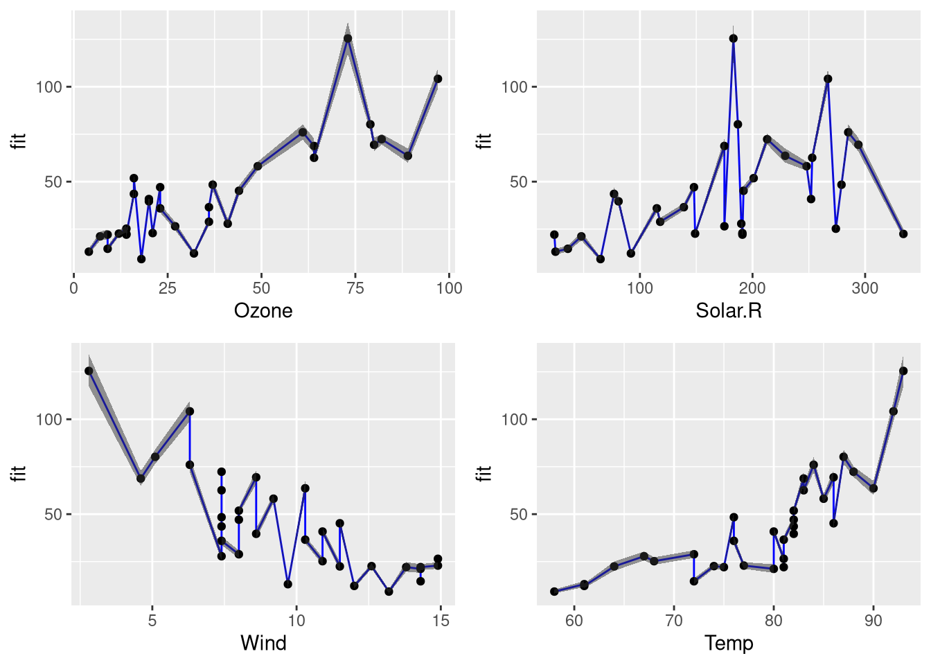
Lamentable
Your postal service has not been submitted. Please return to the class and brand certain that all fields are entered. Thank Y'all!
Source: https://www.datascienceblog.net/post/machine-learning/interpreting_generalized_linear_models/
0 Response to "How to Read Glm Output in R"
Post a Comment